Figures 4 and 5 - Visualizing Module Events and Temporal Use for Certified and Non Certified Students
This R Markdown script reproduces Figure 4 and 5 from the paper, Ginda, M., Richey, M. C., Cousino, M., & Börner, K. (2019). Visualizing learner engagement, performance, and trajectories to evaluate and optimize online course design. PloS one, 14(5), e0215964.
The visualization documented here use analytic results for the MITxPro course, Architecture of Complex Systems (MITProfessionalX+SysEngxB1+3T2016), Fall 2016, with the edX Learner and Course Analytics Pipeline. More information about the data used in this visualization is available at Sample Data Index.
Environment Setup
This is an R Markdown document. Markdown is a simple formatting syntax for authoring HTML, PDF, and MS Word documents. For more details on using R Markdown see http://rmarkdown.rstudio.com.
#Clean environment
rm(list=ls())
options(scipen=90)

#Load required packages
require("RCurl")      #Loading data from web
require("grid")       #Visualizations base
require("reshape2")   #Reshape data package
require("colorspace") #ColorSpace color pallete selection
require("ggplot2")    #GGplot 2 graphics library
require("GGally")
Loading Data
The data set loaded as students was created by the script edX-7-studentFeatureExtraction.R. Data represents the overall performance and interaction statistics for each active student in the course, based on their log activity for the full duration of the course.
#Load Sample Data Set D
students <- read.csv(text=getURL("https://raw.githubusercontent.com/cns-iu/edx-learnertrajectorynetpipeline/master/data/dataD.csv",ssl.verifypeer = FALSE), header=T)
str(students)
## 'data.frame': 1565 obs. of 35 variables:
## $ user_id : logi NA NA NA NA NA NA ...
## $ grade : num 0.94 0 0.94 0.83 0.97 0.52 0 1 0.94 0.96 ...
## $ cert_status : Factor w/ 2 levels "downloadable",..: 1 2 1 1 1 2 2 1 1 1 ...
## $ gender : logi NA NA NA NA NA NA ...
## $ yob : logi NA NA NA NA NA NA ...
## $ loe : logi NA NA NA NA NA NA ...
## $ sessions : int 65 22 53 45 54 28 5 24 48 37 ...
## $ days_unq : int 38 12 29 31 28 14 4 18 36 31 ...
## $ mods_unq : int 284 141 291 255 291 150 86 289 289 274 ...
## $ vid_mods : int 46 23 47 47 47 26 12 47 48 37 ...
## $ prb_mod : int 130 64 139 102 139 65 40 139 139 136 ...
## $ oa_mods : int 5 1 5 5 5 2 1 4 5 5 ...
## $ events : int 4110 439 1200 747 954 680 254 900 832 985 ...
## $ vid_events : int 3379 138 497 273 339 315 73 302 285 280 ...
## $ prb_events : int 224 90 271 150 256 133 98 267 225 267 ...
## $ oa_events : int 43 5 47 21 47 13 3 41 47 50 ...
## $ oa_peerAccessEvents: int 9 0 9 3 9 0 0 9 9 9 ...
## $ oa_getPeerEvents : int 18 0 20 6 20 0 0 19 21 26 ...
## $ seqNextEvents : int 66 37 67 64 61 33 23 58 64 64 ...
## $ seqPrevEvents : int 13 0 7 7 12 11 3 5 11 10 ...
## $ seqGotoEvents : int 16 5 18 23 22 14 0 24 0 3 ...
## $ modAccessEvents : int 54 31 54 52 54 32 20 53 54 53 ...
## $ total_time : num 3236 1074 2738 1369 2021 ...
## $ vid_time : num 1724 265 776 436 698 ...
## $ prb_time : num 187 62.7 220.1 96.6 163.1 ...
## $ oa_time : num 200.37 3.88 168.27 12.42 199.32 ...
## $ oa_peerAccessTime : num 5.517 0 47.25 0.467 23.9 ...
## $ oa_getPeerTime : num 107.62 0 100.72 5.43 165.03 ...
## $ seqNextTime : num 462 443 816 347 458 ...
## $ seqPrevTime : num 29 0 27.68 42.73 7.68 ...
## $ seqGotoTime : num 61.55 2.75 103.07 87.1 74.03 ...
## $ modAccessTime : num 443 223 356 344 342 ...
## $ prb_attempts : int 185 85 211 142 217 96 83 202 199 222 ...
## $ prb_correct : int 119 62 122 93 150 58 72 126 121 120 ...
## $ prb_totalPoints : int 128 67 133 97 159 63 74 140 131 132 ...Sample Data E is used for both figures, and is loaded in to the data frame modules. The data was created from 3 sets of results from script edX-6-moduleUseAnalysis.R. Data represents three sets of module interaction statistics for certification groups identified from analysis of edX course’s user certificate data (e.g. all students, certified and uncertified students).
#Load Sample Data Set E
modules <- read.csv(text=getURL("https://raw.githubusercontent.com/cns-iu/edx-learnertrajectorynetpipeline/master/data/dataE.csv",ssl.verifypeer = FALSE), header=T)
##Feature generation and reshaping data for plots
#Scatter 1: plot of unique number of students using a module
#split by different student percentile groups, which are based students'
#final grade. For cross-group comparison, the values are scaled based on the
#proportion of a percentile groups visiting a module.
modules$unq_stu_per<- modules$unq_stu/max(modules$unq_stu)
modules$unq_stu_per.1<- modules$unq_stu.1/max(modules$unq_stu.1)
modules$unq_stu_per.2<- modules$unq_stu.2/max(modules$unq_stu.2)
#Reshape data for scatter plot visualization 1 using melt
#module unique students by certificate group
#Modules with Zero events are not visualized.
mod_unq <- melt(modules[modules$events>0,c(1:9,19:21)], id.vars=c(1:9))
#Scatter 2 set 2: plot the mean number of events per student, based on the
#number of students in a grade percentile group that use a given module.
#Average module events per students visiting a module
modules$events_meanStd <- ifelse(modules$unq_stu>0,modules$events/modules$unq_stu,0)
modules$events_meanStd.1 <- ifelse(modules$unq_stu.1>0,modules$events.1/modules$unq_stu.1,0)
modules$events_meanStd.2 <- ifelse(modules$unq_stu.2>0,modules$events.2/modules$unq_stu.2,0)
#Reshape data for scatter plot
#Modules with Zero events are not visualized
mod_event <- cbind(mod_unq, melt(modules[modules$events>0,c(1:9,22:24)], id.vars=c(1:9))[10:11])
names(mod_event) [10:13] <- c("var1","val1","var2","val2")
mod_event$module.type <- factor(mod_event$module.type)
#Scatter Set 3: plot the mean time spent per student on a module, based on the
#number of students in a grade percentile group that use a given module.
modules$time_meanStd <- ifelse(modules$unq_stu>0,modules$totalTime/modules$unq_stu,0)
modules$time_meanStd.1 <- ifelse(modules$unq_stu.1>0,modules$totalTime.1/modules$unq_stu.1,0)
modules$time_meanStd.2 <- ifelse(modules$unq_stu.2>0,modules$totalTime.2/modules$unq_stu.2,0)
#Reshape data for scatter plot
#Modules with Zero events are not visualized
mod_time <- melt(modules[modules$events>0,c(1:9,25:27)],id.vars=c(1:9))
mod_time <- cbind(mod_unq, mod_time[10:11])
names(mod_time) [10:13] <- c("var1","val1","var2","val2")
mod_time$module.type <- factor(mod_time$module.type)Visualization of Results
Multiplot Layout
The multiplot function allows for multiple visualizations to be added into a single image. The multiplot function for ggplot2 was taken from the Winston Chang. (2017). Cookbook for R. http://www.cookbook-r.com/.
multiplot <- function(..., plotlist=NULL, file, cols=1, layout=NULL) {
  # Make a list from the ... arguments and plotlist
  plots <- c(list(...), plotlist)

  numPlots = length(plots)

  # If layout is NULL, then use 'cols' to determine layout
  if (is.null(layout)) {
    # Make the  panel
    # ncol: Number of columns of plots
    # nrow: Number of rows needed, calculated from # of cols
    layout <- matrix(seq(1, cols * ceiling(numPlots/cols)),
                     ncol = cols, nrow = ceiling(numPlots/cols))
  }

  if (numPlots==1) {
    print(plots[[1]])

  } else {
    # Set up the page
    grid.newpage()
    pushViewport(viewport(layout = grid.layout(nrow(layout), ncol(layout))))

    # Make each plot, in the correct location
    for (i in 1:numPlots) {
      # Get the i,j matrix positions of the regions that contain this subplot
      matchidx <- as.data.frame(which(layout == i, arr.ind = TRUE))

      print(plots[[i]], vp = viewport(layout.pos.row = matchidx$row,
                                      layout.pos.col = matchidx$col))
    }
  }
}
Setting up visualization themes and parameters
Before visualizing the results, themes for the visualization are set for the ggplot2 package. A set of color palettes are added as well.
#Theme for ggplot2
theme_set(theme_light())

##Color Scales and setting for graphs
strip <- c("#DCDCDC") #Grey

#Univariate color scale
#Multi-color univariate color palette for the module type variables
#Dark blue to yellow green
pal1 <- function (n, h = c(360, 45), c. = c(17, 100), l = c(2, 76),
                  power = c(2.53333333333333, 1.6), fixup = TRUE, gamma = NULL,
                  alpha = 1, ...)
                  {
                    if (!is.null(gamma))
                      warning("'gamma' is deprecated and has no effect")
                    if (n < 1L)
                      return(character(0L))
                    h <- rep(h, length.out = 2L)
                    c <- rep(c., length.out = 2L)
                    l <- rep(l, length.out = 2L)
                    power <- rep(power, length.out = 2L)
                    rval <- seq(1, 0, length = n)
                    rval <- hex(polarLUV(L = l[2L] - diff(l) * rval^power[2L],
                                         C = c[2L] - diff(c) * rval^power[1L], H = h[2L] - diff(h) *
                                           rval), fixup = fixup, ...)
                    if (!missing(alpha)) {
                      alpha <- pmax(pmin(alpha, 1), 0)
                      alpha <- format(as.hexmode(round(alpha * 255 + 0.0001)),
                                      width = 2L, upper.case = TRUE)
                      rval <- paste(rval, alpha, sep = "")
                    }
                    return(rval)
                  }

#Color Scales for Module Types
modColors <- pal1(4)
modColors <- modColors[c(2,1,3,4)]
Figure Labels
##Label groups
#Certification Groups
userGrps <- as_labeller(c('unq_stu_per' = paste0("All students (", length(students$user_id)," students)"),
                           'unq_stu_per.1'  = paste0("Certificate granted, grades between 100%-70% (",
                                                     length(students[students$grade>=.7,]$user_id)," students)"),
                           'unq_stu_per.2'  = paste0("No certification but active, with grades less than 70% (",
                                                     length(students[students$grade<.7,]$user_id)," students)")))
userGrps2 <- as_labeller(c('unq_stu_per' = paste0("All students\n(", length(students$user_id)," students)"),
                          'unq_stu_per.1'  = paste0("Certificate granted\n(",
                                                    length(students[students$grade>=.7,]$user_id)," students)"),
                          'unq_stu_per.2'  = paste0("No certification active\n(",
                                                    length(students[students$grade<.7,]$user_id)," students)")))
modType <- as_labeller(c("html+block" = "HTML/Text\nModule",
                         "openassessment+block" = "Open Assessment\nModule",
                         "problem+block" = "Problem\nModule",
                         "video+block"  = "Video\nModule"))
modLed <- c("HTML/Text\nModule", "Open Assessment\nModule", "Problem\nModule","Video\nModule")
Set vertical lines found in figure
vline <- as.data.frame(unique(mod_unq$L1))
names(vline)[1] <- "L1"
vline$mod <- NA
for(i in 1:nrow(vline)){
  vline[i,]$mod <- max(mod_unq[mod_unq$L1==vline[i,1],]$order)
}
Figure 4 Scatter Plot of Overall Module Use and Unique Number of Student Users
ggplot(mod_unq, aes(x=mod_unq$order,y=mod_unq$value))+
    geom_vline(xintercept=vline[1:nrow(vline)-1,2],linetype="dashed") +
    geom_point(aes(colour=mod_unq$module.type)) +
    scale_colour_manual(values=modColors, labels=modLed) +
    labs(y="Percent of Students Interacting\nwith a Course Module",x="Course Module Sequence") +
    facet_wrap( ~ variable, nrow=3,
                strip.position="top",
                labeller =userGrps) +
    theme(legend.position="bottom",
          legend.title=element_blank(),
          strip.background = element_rect(fill=strip),
          strip.text=element_text(color = "Black"))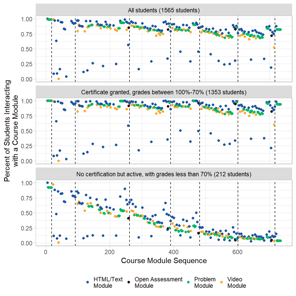
Figure 5 Average Events per Module by Students in Percentile Groups
Fig 5A Mean Number of Events per Html/Text Module
p1 <- ggplot(mod_event[mod_event$module.type=="html+block",], aes(x=order,y=val2)) +
        geom_vline(xintercept=vline[1:nrow(vline)-1,2],linetype="dashed") +
        geom_point(aes(colour=module.type, size=val1)) +
        scale_size(range = c(0, 2.5)) +
        scale_colour_manual(values=modColors[1]) +
        labs(y="Mean Interaction Events per Student") +
        theme(plot.title = element_text(hjust = 0),
              legend.position="none",
              strip.background = element_rect(fill=strip),
              strip.text=element_text(color = "Black"),
              axis.title.x = element_blank()) +
        facet_wrap( ~ var1, nrow=4, strip.position="right", labeller =userGrps2)
p1 + xlab("Course Module Sequence")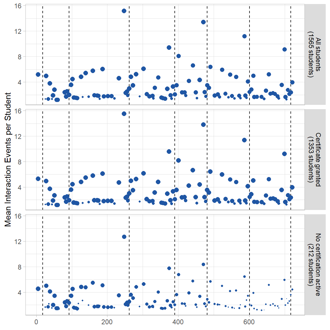
Fig 5B Mean Number of Events per Video Module
p2 <- ggplot(mod_event[mod_event$module.type=="video+block",], aes(x=order,y=val2)) +
        geom_vline(xintercept=vline[1:nrow(vline)-1,2],linetype="dashed") +
        geom_point(aes(colour=module.type, size=val1)) +
        scale_size(range = c(0, 2.5)) +
        scale_colour_manual(values=modColors[4]) +
        theme(plot.title = element_text(hjust = 0),
              legend.position="none",
              strip.background = element_rect(fill=strip),
              strip.text=element_text(color = "Black"),
              axis.title = element_blank()) +
        facet_wrap( ~ var1, nrow=4, strip.position="right", labeller =userGrps2)
p2 + labs(x="Course Module Sequence",
             y="Mean Interaction Events per Student")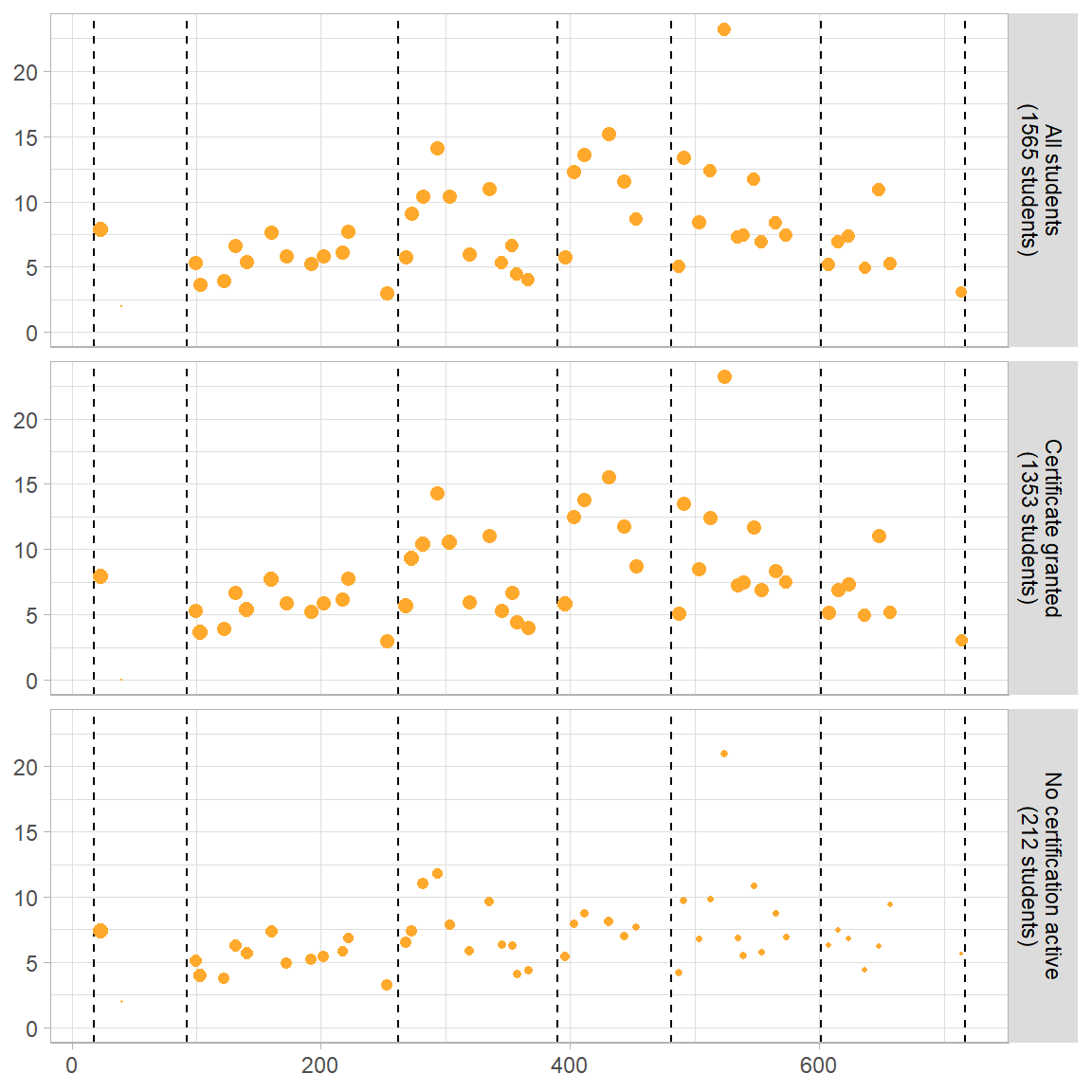
Fig 5C Mean Number of Events per Problem Module
p3 <- ggplot(mod_event[mod_event$module.type=="problem+block",], aes(x=order,y=val2)) +
        geom_vline(xintercept=vline[1:nrow(vline)-1,2],linetype="dashed") +
        geom_point(aes(colour=module.type, size=val1)) +
        scale_size(range = c(0, 2.5)) +
        scale_colour_manual(values=modColors[3]) +
        labs(x="Course Module Sequence",
             y="Mean Interaction Events per Student")+
        theme(plot.title = element_text(hjust = 0),
             legend.position="none",
             strip.background = element_rect(fill=strip),
             strip.text=element_text(color = "Black")) +
        facet_wrap( ~ var1, nrow=4, strip.position="right", labeller =userGrps2)
p3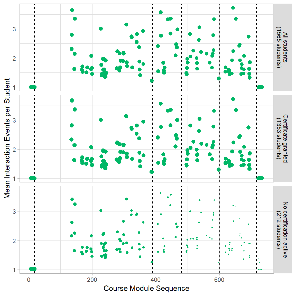
Fig 5D Mean Number of Events per Open Assessment Module
p4 <- ggplot(mod_event[mod_event$module.type=="openassessment+block",], aes(x=order,y=val2)) +
        geom_vline(xintercept=vline[1:nrow(vline)-1,2],linetype="dashed") +
        geom_point(aes(colour=module.type, size=val1)) +
        scale_size(range = c(0, 2.5)) +
        scale_colour_manual(values=modColors[2]) +
        labs(x="Course Module Sequence") +
        theme(plot.title = element_text(hjust = 0),
              legend.position="none",
              strip.background = element_rect(fill=strip),
              strip.text=element_text(color = "Black"),
              axis.title.y = element_blank()) +
        facet_wrap( ~ var1, nrow=4, strip.position="right", labeller =userGrps2)
p4 + ylab("Mean Interaction Events per Student")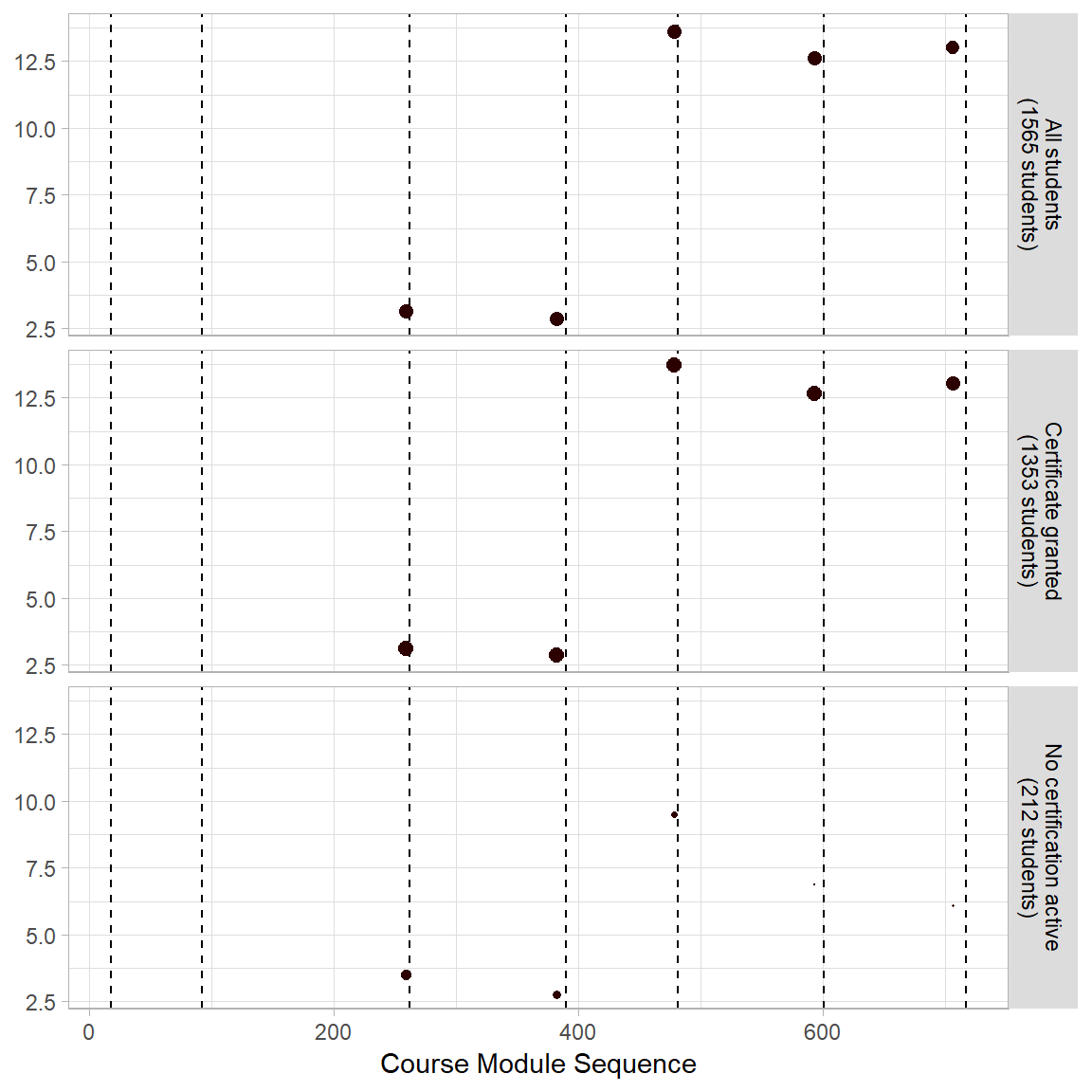
Fig 5 Composite
#Final Layout
multiplot(p1 + ggtitle("A")+ theme(plot.title = element_text(hjust = 0)),
          p3 + ggtitle("B")+ theme(plot.title = element_text(hjust = 0)),
          p2 + ggtitle("C")+ theme(plot.title = element_text(hjust = 0)),
          p4 + ggtitle("D")+ theme(plot.title = element_text(hjust = 0)),cols=2)